Football-Data's revenues come from losses accrued by customers of advertised bookmakers. Nearly all bettors lose in the long run. Users taking advantage of any advertised welcome offer should familiarise themselves with the bookmaker's T&Cs. Any information appearing on this website, including references to winning, profit, beating odds/bookmakers etc. should not be considered professional advice or a recommendation to bet or gamble. Furthermore, the small proportion of customers considered by bookmakers to be sufficiently skilled at beating their prices may find their stakes restricted or have their accounts closed. Both the UK Government and bookmakers alike maintain that betting and gambling in the UK should be considered a form of entertainment only and not a trade to make money. Please gamble responsibly. NEVER risk what you cannot affort to lose. BeGambleAware.

Testing the Reliability of my Betting Record Test Formula

In my second book How to Find a Black Cat in a Coal Cellar: The Truth about Sports Tipsters and more recently in my third book Square & Sharps, Suckers and Sharks: The Science, Psychology and Philosophy of Gambling I published a simple method for how to test the profitability of your betting record, and specifically how likely it could arise by chance. A summary of the material can be found in Pinnacle's Betting Resources. I have also made the test available as a basic Excel calculator which you can download from Football-Data.

Recently, Marius Norheim, CEO of the betting analysis tool TrademateSports (which effectively automates my Wisdom of Crowds betting system) questioned how robust or reliable my test actually is. I must confess that save a little bit of testing at the time I developed the methodology, I undertook no formal examination of its validity. This is the purpose of this article. For those who may struggle to follow my discussion, I would urge you to familiarise yourself with the original material on my use of the t-test for testing betting histories in the sources already referred to.

Let's being by explaining again what the test is. Based on the student's t-test for statistical significance (of whether a sample mean deviates significantly from the population mean), the method simply compares a bettor's return from a sample of bets to a theoretical expectation defined by the market they're betting in, and analyses whether the difference is statistically significant. If it is, we may reject the null hypothesis, which assumes that observed profits and losses are purely the result of chance, in favour of a different one. The t-test does NOT tell us what that new hypothesis would be, nor the probability of it being valid, but the underlying presumption is that any statistically significant return by the bettor would be the result of skill. The t-statistic or t-score is really just a measure of the departure of the observed sample mean away from expected population mean, and is defined by the following equation:

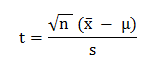
where x̄ is the sample mean (the average profit per bet), μ is the population mean (the random profit expectation), s is the sample standard deviation in profits and losses of the betting history and n is the sample size (the number of bets).

I've previously made a case for setting μ = 0. Using an odds comparison allows a bettor to compare prices across a number of bookmakers and pick the best one. Typically this allows a bettor to more or less eliminate the bookmaker's margin; that is to say on average they are achieving roughly fair odds, with a profit expectation of 0.

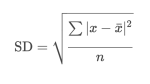
If nothing else this simplifies the t-statistic equation, since we now only have to worry about x̄, n and s. x̄ and n are easily determined: just count your profit and divide it by the number of your bets. But what about s, the standard deviation (or variation), in your sample of profits and losses? A standard deviation is easily calculated in a spreadsheet package like Excel (=STDEV), but it would be handy to be able to calculate it by other means.

The standard deviation measures the spread of the data about the mean value; in this case the sample mean is our yield or x̄. The standard deviation is specifically the mean of the sum of the squares of the differences between actual profits and the sample mean. Suppose be had 10 bets at odds of 3.00, with 5 winners and 5 losers. The 5 winners would have profits of 2 and the 5 losers losses of -1. For each profit or loss, we subtract the sample mean (in this case a profit of 5 divided by 10 bets = 0.5). We then square each result, add them all up, divide this result by n, the number of bets and finally take the square root. The formula looks like this.

So far this is just standard statistical theory. But really it's a bit of a pain in the backside to have to do all of that mathematics manually. Fortunately, it's possible to derive a simpler formula from the one above by counting the number of wins and losses in the betting history for cases where all of the bets have the same odds. It is shown below.

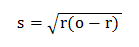
r is the decimal return on investment (or x̄ + 1) and o is the betting odds. Since we always know r and o, it's pretty straightforward to calculate s.

The final steps are to insert this formula for s into the equation for the t-statistic above and then to calculate a p-value, the probability that our betting history could have happened by chance, assuming nothing else like skill is influencing it. This can be done in Excel using the =TDIST function, or by referring to t-test tables. Since we're only really interested in profitability, I have typically used the one-tailed test.

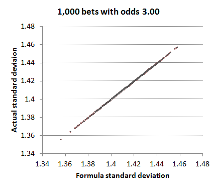
We can test how reliable my formula is for the standard deviation in the profits/losses of a betting history by simulating a number of betting histories (using a random number generator to determine the results assuming a profit expectation of 0) and comparing the actual standard deviations for each history (calculated by Excel) with the standard deviations calculated via this formula. I've done this for a betting history of 1,000 wagers, each with odds of 3 and plotted the results below. Since standard deviation will vary depending on the return (r), we will have a 1,000 different points. In this simulation, r varied between 0.858 and 1.146. (For the case r = 1, the standard deviation formula will give a value of √2 or about 1.41; it will be lower when r < 1 and higher when r > 1.) We can see how the formula standard deviations are a perfect match for the actual standard deviations. This is unsurprising since all the odds were the same.

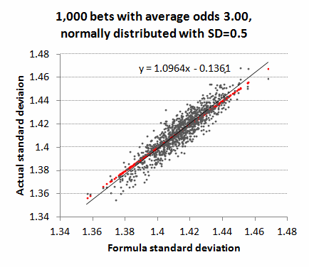
What if we now vary the odds a bit about an average of 3? To achieve this I randomised the betting odds using a normal distribution around an average of 3.00 and a standard deviation of 0.5. The shortest odds were 1.41 and the longest were 4.69. r varied between 0.859 and 1.191. This time there is not quite a perfect match. The red dots mark the idealised correlation, whilst the grey dots show how actual standard deviation varies with the formula standard deviation. The thin black line shows the average trend of correlation between formula and actual standard deviations. You can see it doesn't quite follow the red line having a gradient slightly greater than 1.

What impact does this deviation in the expected (or formula) standard deviations from those actually observed have on the p-values? Despite the imperfect correlation between formula standard deviation and actual standard deviation on account of the variance in the betting odds, p-values estimated from the formula method are still a very close match for those calculated using the actual standard deviations.

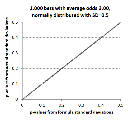
This reliability persists for p-values that we are most interested in, namely those less than 0.05 where statistical significance of a betting history begins to emerge.

Arguably, however, normally distributed betting odds are not very representative of a typical betting record with about half the odds shorter than 3 and half longer than 3. Next, I used a uniformly random set of win percentages restricted between 5% and 95% to build a set of 1,000 odds, more representative of typical betting markets. Whilst still maintaining an average of 3, the majority (73%) were shorter than 3.00 whilst the minority (27%) were longer than 3.00. The shortest odds were 1.07, the longest 19.7, with a standard deviation of 2.86. Returns varied between 0.854 and 1.142 It's probably unlikely that the majority of bettors would have such a varied sample of betting odds. Most tend to focus on particular markets where the range of odds is narrower (for example Asian handicap or 1X2 in football), but the aim here is to test robustness of my standard deviation formula to extreme scenarios.

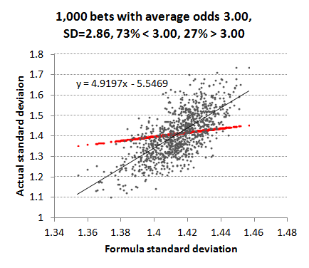
This time the deviation of actual standard deviations from their formula counterparts is far more marked. Whilst the average is still around 1.41 (or the square root of 2 as predicted by the formula when r = 1), there is both a wide spread in the actual data and a markedly different trend line (gradient = 4.91). Essentially, my formula is underestimating the actual standard deviations when r > 1 and overestimating them when r < 1. Why should this be? Well, In a sample where there are varying odds, the influence of good or bad luck will be greater the longer the odds. One lucky winning bet at long odds, for example, will increase the actual standard deviation in the profits/losses history far more than the formula equivalent, which is just assuming that all the odds are the same (in this case 3.00).

Let's take a look again at what impact this imprecision has on p-values. Clearly it's not a perfect correlation but it's far from invalidating the use of the formula.

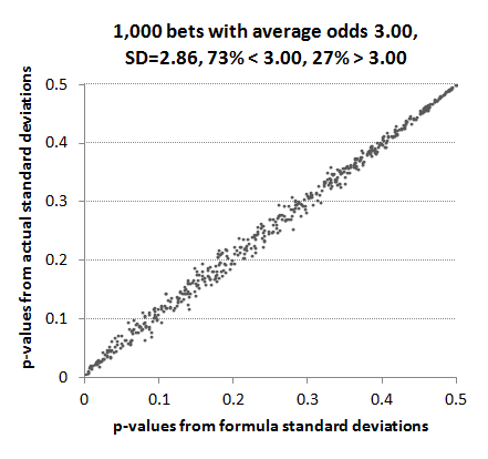
This is unsurprising if we look again at the y-axis scale in the previous chart. Although the correlation between formula and actual standard deviation for varying returns diverges markedly from that predicted by the formula, there is still a fairly narrow range of actual standard deviations. Most fall between 1.25 and 1.55. Since the t-statistic is fairly insensitive to small changes in the standard deviation, it is still useable. For example, the formula-predicted standard deviation for a record of 1,000 bets with average odds 3.00 and returns 1.1 would be 1.446 for a p-value of 0.0145 (1.45%). Suppose instead the standard deviation was 1.346 or 1.546. The p-values would be 0.0095 (0.95%) and 0.0205 (2.05%) respectively.

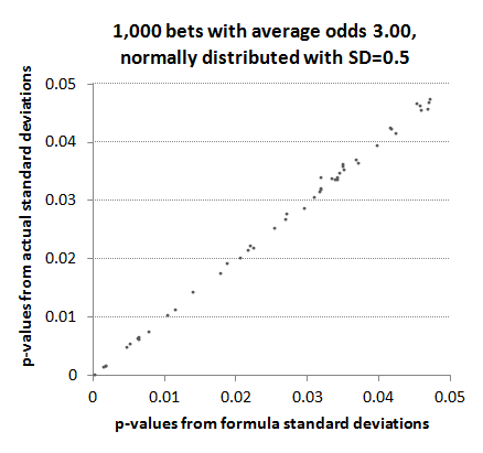
The final chart shows the p-value correlation between formula and actual figures for values less than 0.1.

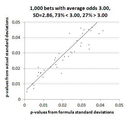
We can see that the formula method marginally underestimates the p-value, and hence marginally overestimates any statistical significance we might attribute to profitable records arising from anything other than chance. Given that the shortest p-values arise for the biggest returns this is unsurprising since we've already seen that actual standard deviations are likely to be higher than those predicted by the formula. The smaller the standard deviation, the larger the t-statistic and the smaller the p-value.

Nevertheless, despite the failure of the formula to perfectly reproduce actual standard deviations in the profits and losses of betting histories with real world variations in betting odds, the method of using the average odds to estimate them is arguably robust enough to yield meaningful ballpark estimates of the statistical significance for all but the most odds-variable of betting records. After all, that was all the formula was meant to do. However, if in doubt just use your actual betting history standard deviation rather than the one estimated by the formula.