Football-Data's revenues come from losses accrued by customers of advertised bookmakers. Nearly all bettors lose in the long run. Users taking advantage of any advertised welcome offer should familiarise themselves with the bookmaker's T&Cs. Any information appearing on this website, including references to winning, profit, beating odds/bookmakers etc. should not be considered professional advice or a recommendation to bet or gamble. Furthermore, the small proportion of customers considered by bookmakers to be sufficiently skilled at beating their prices may find their stakes restricted or have their accounts closed. Both the UK Government and bookmakers alike maintain that betting and gambling in the UK should be considered a form of entertainment only and not a trade to make money. Please gamble responsibly. NEVER risk what you cannot affort to lose. BeGambleAware.

Profit Expectations of a Sports Bettor

Those of you who read my articles regularly, and certainly those who have read my latest book Squares & Sharps will know that I sell a rather depressing message about sports betting: almost all of what happens is luck. One of the most significant pieces of evidence I have published to support my view is the analysis of data kindly made available by the tipster supermarket Pyckio. Plotting the distributions of over 6,000 tipsters who had collectively issued over 1 million tips during an 8-month period (June 2014 to February 2015), their performances were almost identical to what would be expected to happen purely randomly. I'm not naïve to believe there are no tipsters or bettors capable of finding a genuine profitable expectation through their skill which is sustainable over the long term. After all, the reason I'm in this business at all was through the inspiration I gained from someone who most definitely was. However, my view is that there really aren't very many, most likely less than 1% and conceivably less than 0.1% or even 0.01%.

In this article, I want to revisit that Pyckio data and break it down into different odds ranges to investigate the different ranges of performances and draw some conclusions about likely profit expectations. In keeping with the original analysis, my assumption will be that nearly all of what happens is due to chance. Of course, for the few of you where that is not the case, the same rules of statistical variance still apply. If you have a bit of additional skill on your side, that should be regarded as a bonus which will see you right in the long run. But even for you, chance will dominate short to medium term expectations, and hence it is useful to take a look at what those might be.

In my original article analysing Pyckio tipsters, I plotted their performances by t-scores. This helped me compare different lengths of betting history and tipsters betting different odds in a risk-adjusted way. However, it's not as intuitively understandable and given that this time I want to compare and contrast the ranges of performances for different odds, plotting yields is my preferred option this time.

For the purposes of the analysis I've only considered tipsters which have had at least 100 tips for a particular chosen odds range. I opted to analyse 4 different odds ranges: Odds less than 1.50, odds from 1,5 to less than 2, odds 2 to less than 3, and odds 3 and over. Typically I would prefer to analyse a greater range, for example odds 3 to 5, 5 to 10 and over 10, but there simpler weren't enough tipsters and tips to make the analysis meaningful.

There were 576 tipsters in my dataset who issued at least 100 tips with odds less than 1.50, accounting for a total of 185,841 tips. Their yields from these are plotted in the distribution below (blue line), with the x-axis divided into 1%-yield divisions. The total yield for all tips was -0.75%. 42% of the tipsters were profitable, with a standard deviation of 4.1%. [The standard deviation of a sample is simply a statistical measure for how much the data in that sample vary about a mean; the bigger the variance the bigger the standard deviation.] For these short odds, the aggregated yield is pretty close to Pinnacle's betting margin at those prices (because of the favourite-longshot bias), and remember that all these tips were issued at Pinnacle prices.

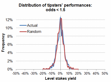
The actual distribution of tipsters' yields is contrasted to a distribution that occurred when assuming a random settlement of bets (using Excel's random number generator to decide how a bet would be settled (the red line). For this single random run, the average aggregated yield was -0.77% and the standard deviation in tipsters' yields was 4.2%, figures almost identical to the actual data. Because Excel's random number generator will produce to a normal distribution, we can say with confidence that the actual distribution of tipsters performances from betting odds less than 1.50 is pretty close to normal, and therefore random.

Knowing the standard deviation then allows us to make predictions about what to expect, simple by using a normal distribution calculator, either Excel's own formula (NORMDIST) or a simple online version. For example, we can predict that tipsters without skill betting Pinnacle odds less than 1.5 making several hundred tips will achieve a yield of 4.5% or better about 10% of the time, and 9% or better about 1% of the time, just by chance. If you know the average and standard deviation, and you know your possible betting histories are normally distributed, you can pretty much estimate any possible scenario.

The next chart shows the performances of the 1078 tipsters issuing 408,105 tips with odds 1.5 up to but not including 2. The aggregated yield was -2.1%, a bit worse than that expected given Pinnacle's margin for those odds, whilst 33% of the tipsters were profitable. Again actual performances are contrasted to a randomised run (aggregated yield = -1.3%). Again, there's little difference.

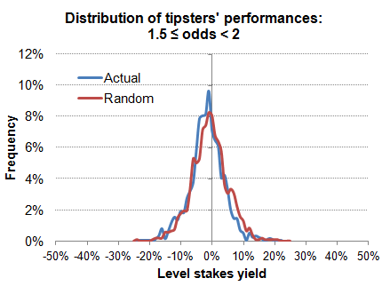
Crucially the standard deviations are almost the same again, 5.8% to 2 significant figures for both actual and random distributions. This is a little higher than for the first distribution with shorter odds. We should not be surprised. Longer odds means more uncertainly, means more variance and a bigger range of outcomes. This time about 3% of tipsters will make a yield of 9% from a few hundred Pinnacle wagers, despite the aggregated average actually being lower.

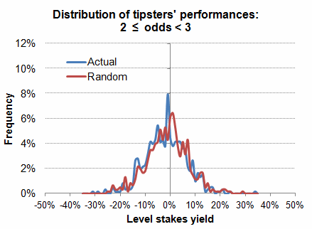
The third chart shows the actual and random distributions for odds 2 up to but not including 3. Ignore the wavy nature of the distribution line, this is simply on account of smaller volume of data to analyse. Aggregated actual and random yields were -2.3% and -1.6% respectively from 173,973 tips by 603 tipsters. 38% of tipsters were profitable. Standard deviations were 8.3% for both, considerably higher than for the lower odds ranges. Now, as many as 9% of tipsters can be expected to make a 9% yield after several hundred Pinnacle tips.

Finally, the last chart shows the performances of 197 tipsters issuing at least 100 tips with odds of 3 or more for a total of 46,887 tips. Again, the even smaller amount of data available to analyse renders the plot very imprecise, but the general normal bell-shaped curve can still be seen underlying it. Aggregated yield was -3.2% (-2.1% random) with 38% of tipsters profitable.

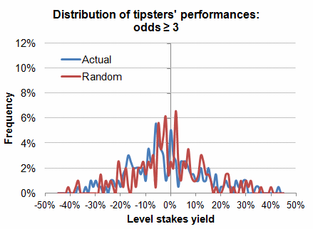
Standard deviations for actual and random distributions were 14.6% and 14.4% respectively. As many as 20% of tipsters could now be expected to make a 9% yield after a few hundred tips, such is the variance in outcomes betting at these longer odds. No doubt, if I had been able to analyse properly odds of 10 and over the variance would have been even greater still.

The purpose of showing these plots is to illustrate two important things. Firstly, across a variety of odds, almost everything that happens is because of chance. Secondly, the range of possible performances increases significantly as the probability of individual bets winning decreases. I purposely plotted each of the four charts using the same x- and y-scales to allow you to compare and contrast the underlying shapes. Essentially the longer the odds we bet at, the greater the possibility of doing really well. Unfortunately, there is also a greater possibility of doing really badly. Gambling is about risk and reward, You want bigger rewards? You gotta take bigger risks to get them.

There is one major caveat with this analysis here. I've grouped together tipsters with vastly varying histories. Some had 100 tips, some had thousands. It's pretty obvious that for a tipster with only luck in his side, he's less likely to be showing any sort of profit after 1,000 bets than after 100 bets. Such is the nature of the law of large numbers. This was the reason my original analysis published in my book used t-scores and not yields. Fortunately, this variation in betting history length hasn't proven to be too problematic in illustrating these broad conclusions.

However, we can of course idealise our profit expectations simply by running some Monte Carlo analyses with different numbers of bets/tips and different odds. I've done this for 3 different bet totals (100, 1,000 and 10,000) and for 6 different betting odds (1.25, 1.5, 2, 3, 5 and 10) for a total of 18 model scenarios (each with a 10,000-iteration Monte Carlo) and where every wager has an assumed expected value equivalent to a margin of -2.5% (for simplicity I've ignored the influence of the favourite-longshot bias here). The standard deviations in yield are shown in the table below.

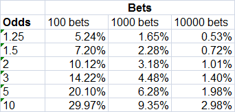
The figures illustrate again how standard deviation decreases with decreasing odds (or increasing bet win probability). In fact, the standard deviation decreases in direct proportion to the logarithm of the bet win probability, as the next chart illustrates (the x-axis here is logarithmic).

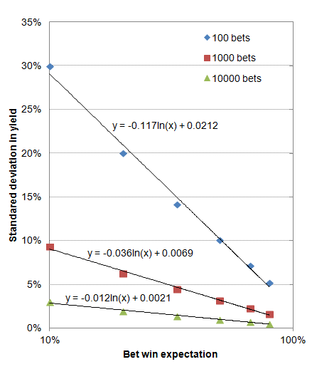
These figures (and the chart above) confirm the law of large numbers which states that an average (in this case the yield) obtained from a number of trials (in this case profits and losses in a betting history) will tend closer towards the expected value as more trials are performed. That's simply another way of saying that the variance (and hence standard deviation) in a sample of those averages (yields) will decrease as the trial (bet) number increases.

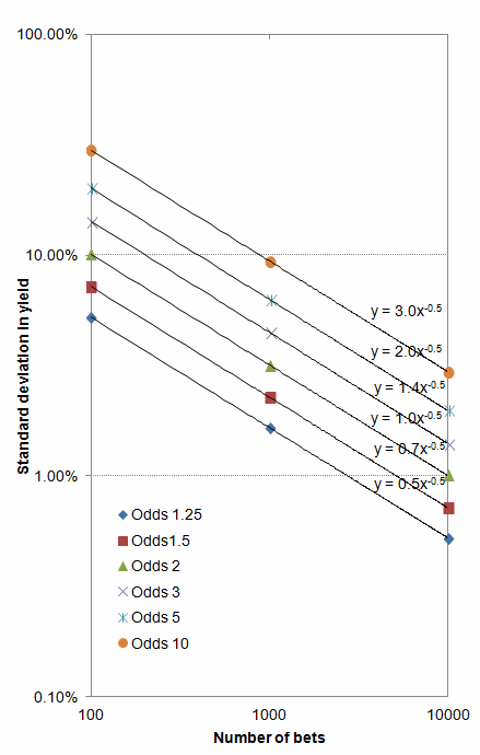
Take a look again at the table of standard deviations and notice how the figures for 10,000 bets are 10 times smaller than the figures for 100 bets. This is no coincidence. In fact, the relationship between bet history size and standard deviation in possible yields follows a power law. When describing such a relationship graphically you will see a straight line relationship on a log-log plot. I've done this below for the 6 different betting odds scenarios. For each, the standard deviation in possible yields is inversely proportional to the square root of the number of bets.

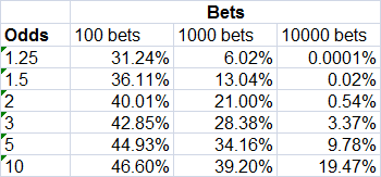
How do these standard deviations help us determine how likely it is to achieve different levels of profitability? Let's return to the normal distribution calculator. Consider the case of 1,000 bets of odds 2.00. The standard deviation in possible yields is 3.18%. With an expected yield of -2.44% (given by 1/1.025 - 1 where 1.025 is the bookmaker's margin), the probability of being in profit is 22.2%, whilst the probability of showing a 5% yield is about 1%. After 10,000 bets however, the law of large numbers gets to work. Now the probabilities of break even and 5% yield are just 1% and 1-in-10 trillion. The full set of figures for breaking even for all 18 scenarios are shown below.

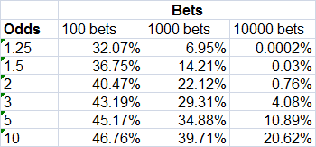
You might be looking at that table and thinking, well I've got a much better chance of being in profit after a load of bets if I bet much longer odds. That is certainly the case, and is a consequence of the greater variance and uncertainy with longer odds. But the flip side is also true: you've also got a much greater chance of showing heavier losses. The final table below illustrates the probabilities of showing a -5% yield.

Some of this may seem rather theoretical. But knowing the relationship between the size of our bet history and the variability in possible yield outcomes can help us make predictions of what to expect in the future based on an existing history of bets. By using Monte Carlo to reveal this power law relationship, we can help ourselves determine how long it might take to be sure any advantageous value expectation we hold will be revealed in sustainable profitability, or conversely if we don't hold any, how long it will take us to realise it's time to give up betting.